In this post I’ll demonstrate generating UTM grid labels in the QGIS print composer with formatting that promotes relevant information is a consistent way. Printing the full 6/7 figure reference on each grid interval is unnecessary and frequently unhelpful as often we need to read off/locate a 3 figure reference.
Abbreviated UTM Grid References?
When reading a UTM grid reference on a typical 1:25000-50000 scale topographic map featuring a 1km grid interval, a 6-figure grid reference (3 figures for Eastings and 3 for Northings) describes a location to 100m precision and is typically sufficient for locating a position on the map.
A full UTM grid reference describes a position to 1m precision. Therefore, we typically highlight the significant figures on the map for ease of using a 6 figure reference with the map.
Of course we might still want to know the full reference, so there should be some full grid references given. For consistency, these are often placed in the corners of the map. To find the full reference for a shortened reference, go to the left/bottom of the map and count up.
Here’s an example from a local state-issued topographic map:

QGIS print composer has the ability to draw and label a UTM grid. However, it’s styling options are somewhat limited out-of-the-box, restricted to a full reference at each interval.
Rendering sub/superscript labels
Most unicode-compatible fonts contain glyphs for superscript and subscript representation of ordinals:
012345678901234567890123456789
QGIS does not handle superscript/subscript formatting internally, but we can achieve the same effect by transposing the numbers with their unicode sub/super-script equivalent characters. Note that this technique is limited to the common Arabic numerals 0-9.
In the Python code below the function UTMFullLabel performs two operations:
- Determine the non-significant figures of the reference to conditionally format. The index of those figures in the reference depends on whether the label is an Easting (6) or Northing (7).
- Transpose those figures to subscript
The function UTMMinorLabel merely returns the significant figures. There are two functions as two separate grids are defined in the print composer, and using two formatting functions avoids also handling grid interval logic in Python.
from qgis.utils import qgsfunction
from qgis.gui import *

@qgsfunction(args="auto", group='Custom')
def UTMMinorLabel(grid_ref, feature, parent):
 return "{:0.0f}".format(grid_ref)[-5:-3]

@qgsfunction(args="auto", group='Custom')
def UTMFullLabel(grid_ref, axis, feature, parent):
 gstring="{:0.0f}".format(grid_ref)
 rstr = gstring[-3:] #3 last characters
 mstr = gstring[-5:-3] #the 5th-4th characters
 #either the 1st or 1-2 for the most sig figs depending if there 6 or 7 digits
 lstr = ''
 if (len(gstring) == 6):
 lstr = gstring[0] #first 2 digits
 elif (len(gstring) == 7):
 lstr = gstring[0:1]
 else:
 return str(len(gstring))
 return "{0}{1}{2}m{3}".format(sub_scr_num(lstr),mstr,sub_scr_num(rstr),'E' if axis == 'x' else 'N')

def sub_scr_num(inputText):
 """ Converts any digits in the input text into their Unicode subscript equivalent.
 Expects a single string argument, returns a string"""
 subScr = (u'\u2080',u'\u2081',u'\u2082',u'\u2083',u'\u2084',u'\u2085',u'\u2086',u'\u2087',u'\u2088',u'\u2089')
 outputText = ''
 for char in inputText:
 charPos = ord(char) - 48
 if charPos <0 or charPos > 9:
 outputText += char
 else:
 outputText += subScr[charPos]
 return outputText
For superscript formatting the transposition is:
supScr = (u'\u2070',u'\u00B9',u'\u00B2',u'\u00B3',u'\u2074',u'\u2075',u'\u2076',u'\u2077',u'\u2078',u'\u2079')
Now that we can generate long and short labels they need to be placed appropriately on the grid:
- Full labels for the grid crossings closest to the corners of the map
- Abbreviated labels for all other grid positions
This logic is handled in QGIS’ expression language. This could be handled in Python too by passing in the map extent. In English, it is basically performing the procedure:
- Get the extent (x/y minimum and maximum values) of the map.
- Test which is closer to the map boundary
- The axis minimum/maximum plus/minus the grid interval
- The supplied grid index being labelled
- Neither – they’re coincident (i.e. the first label is at the axis)
If the value supplied is closer to the map boundary or they’re co-incident then this must be the first label and should be rendered as a full reference.
CASE
  WHEN  @grid_axis = 'x' THEN
    CASE
      WHEN x_min(map_get(item_variables('main'),'map_extent')) + 1000 >= @grid_number THEN  UTMFullLabel( @grid_number, @grid_axis)
      WHEN x_max(map_get(item_variables('main'),'map_extent')) - 1000 <= @grid_number THEN  UTMFullLabel( @grid_number, @grid_axis)
      ELSE UTMMinorLabel(@grid_number)
    END
  WHEN @grid_axis = 'y' THEN
    CASE
      WHEN y_min(map_get(item_variables('main'),'map_extent')) + 1000 >= @grid_number THEN UTMFullLabel( @grid_number, @grid_axis)
      WHEN y_max(map_get(item_variables('main'),'map_extent')) - 1000 <= @grid_number THEN UTMFullLabel( @grid_number, @grid_axis)
      ELSE UTMMinorLabel(@grid_number)
    END
END
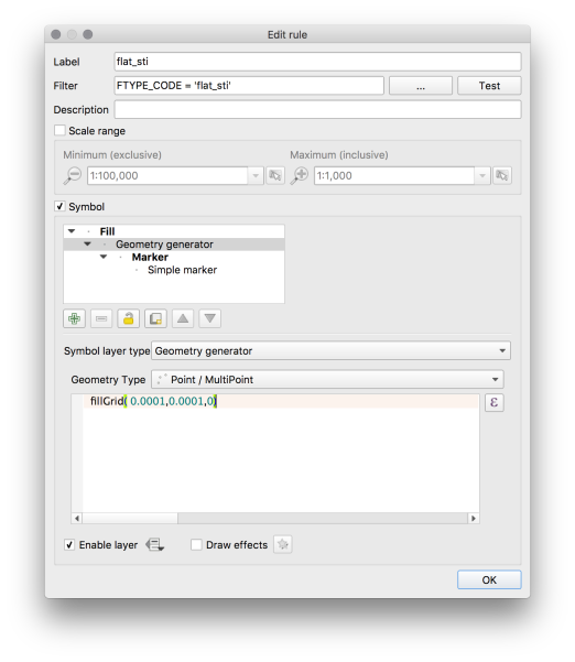
Finally to tie all of this together, in the Print Composer three grids are defined:
- 1000m UTM grid for lines and labels
- 1000m UTM grid for external tick marks
- 1 arc-second interval secondary graticule
Two UTM grids are required as QGIS can either draw grid lines or external ticks. Both were desired in this example.

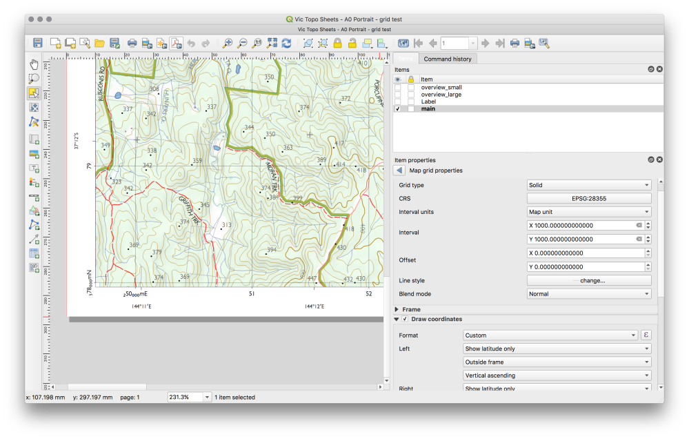
For the grid rendering the labels, set the interval to 1000m, custom formatting as described above and only label latitudes on the left/right and longitudes on the top/bottom.
The formatting of the labels should look something like the screenshot above.
The only thing I haven’t covered here in the interest of clarity is the selective rotation of the Y-axis labels as seen in the state-issued topo map. This could be achieved by using an additional grid and setting the rotation value appropriately.