GIS, Open-Source

Propeller AeroPoints – Offline Processing

Retrieve raw Ublox log files and manually PPK post-process it using RTKLIB 

TLDR

  • AeroPoints upload raw ubx-format log data over clear HTTP to AWS S3.
  • Intercept using mitmproxy/wireshark/tcpdump/whatever
  • Extract binary payload
  • Post-process ubx data in RTKLIB; PPK or PPP mode.
  • Enjoy accurate Ground Control Points.

Propeller AeroPoints are sold as a convenient way of placing Ground Control Points on an aerial imagery survey. You lay them out, turn them on, acquire your imagery and after collecting them, turn them on again in the presence of WiFi. Your data is uploaded to the cloud, and by magic the locations of your control points are given to, they claim, an accuracy of 5cm. $6000 for a set of 10, plus $600/year to keep your subscription to their cloud processing service active.

If Propeller stop paying their AWS bill, or you stop paying your subscription, these things become doorstops.

Long story short, I ended up with a set that someone was too cheap to keep up the subscription on, and I had some survey points I wanted to get at. In a commercial setting I’d pony up, but, $600 to get 10 control points was more than I could justify for a home project. And, philosophically, it’s my data. So, let’s have at it.

Reverse Engineering

So what’s actually going on inside these? Claims of kinematic GNSS accuracy for $600 a unit, and their cloud platform suggest it’s almost certain that low cost components are being used. But which?

GNSS Receiver

The ubiquitous Ublox M8-T module is a likely candidate, though I haven’t taken the foam off the back to actually find out for sure. It seems like a destructive process ripping off the foam backing. The M8T doesn’t perform real time RTK corrections by itself, but it doesn’t matter. As position solutions are being post-processed on Propeller’s cloud service, only raw log data from the receiver is required.

Logging and WiFi

The front panel of the AeroPoint tells us that it contains a part with ID 2AHMR-ESP12S. an ESP12. This is an FCC certified/SMT version of the popular ESP8266 WiFi-SoC, and host of a thousand low power embedded projects due it being available retain for a couple of bucks.

This tells me a few things:

  • They’re using external storage, for the 4GB of log space. My guess is an SD card reader connected over SPI.
  • They’re probably not TLS securing the data upload to the cloud. HTTPS support is known to be flaky on the ESP8266. It doesn’t really have enough memory to store the necessary certificates to validate the certificate chain and your application code.
  • Even if they did get TLS working, they’d also need a full over-the-air upgrade stack, because what if a certificate expires or is revoked? Which means they also need a means of securing the OTA process.

My money is on this thing having baked-in firmware and communication in the clear.

And this is the problem with a lot of “IoT” devices. Poor or no security,  unmaintainable software, consigned to rapid obsolescence.

Admittedly, these are essentially GNSS data loggers that are only network connected for minutes at a time, infrequently. Outside of crypto-ned territory,  if ‘the man’ is your adversary, exploiting a buffer overflow via a man in the middle attack on your data logger’s HTTP client, you already know you need to be not running devices like this on your network. Or at least you should.

For everyone else, the real security risk is academic. Rant over. Moving on.

Extracting GNSS log data

The AeroPoint uploads data to an AWS instance over unsecured HTTP. Intercepting this is trivial. My approach in this instance was to use:

See the mitmproxy documentation for a tutorial.

Ensure you have positively verified that traffic flows are saved and that you can extract the binary payload data from other hosts before attempting this process. Once the data is uploaded, it’s deleted from the AeroPoint.

Setup your Access Point with the WPA settings Propeller require, and power up the first AeroPoint. You should see some back and forth to:

  • groundcontrol.propelleraero.com
  • propeller-data-us-east-1.s3-accelerate.amazonaws.com

The initial API calls acquire an access key for the S3 data upload. You want the multi-megabyte payload of the POST calls to S3. The log data is sent as binary, in raw ubx format, no additional compression or packing.

Now, repeat for as many of the AeroPoints as you have. Refer to the mitmproxy documentation if you’re unsure how to do this.

Post Processing in RTKLIB

As with traffic interception, there’s more than one way to achieve the next step and I’m just going to refer you to the documentation.

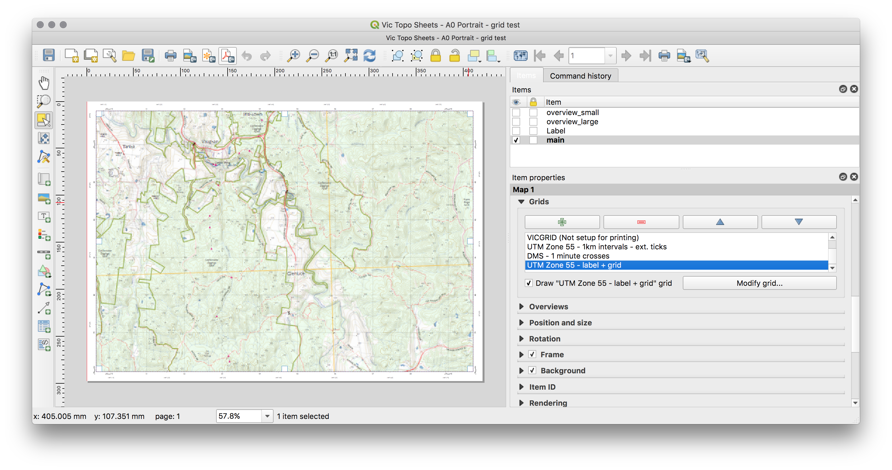
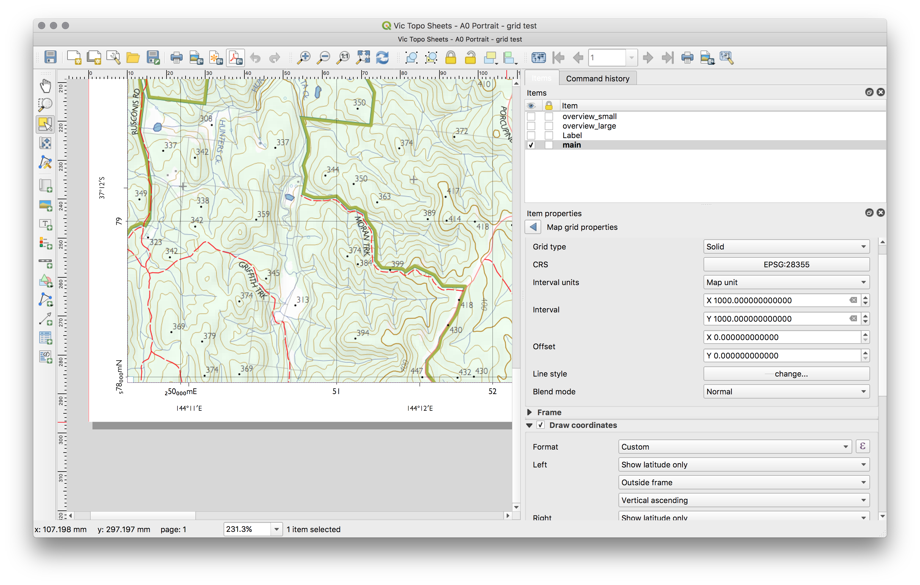
In my case I loaded the ubx data into RTKLIB, and used PPK processing with a local CORS station acting as the base.

The folks at emlid have some good instructions on PPK techniques using RTKLIB. They’ve done a fair amount of work to improve the performance of RTKLIB on low-end hardware too. Check out their RTKLIB fork and their hardware too. Beyond retrieving the log data from their receiver, their process is applicable here.

In my case, I used RINEX logs from the AUSCORS archive (I’m in Australia) for a local CORS station, Fortunately I had a short enough baseline to a public CORS site for high accuracy solutions.

One valuable thing a Propeller subscription buys is access to several commercial  CORS networks.

For additional accuracy, I waited a couple of weeks for the final GPS/GLONASS orbital data to be published and used the following data from IGS:

Final SP3 ephemeris 
File name format: WWWW/igsWWWWD.sp3.Z https://cddis.nasa.gov/Data_and_Derived_Products/GNSS/orbit_products.html 

Final clock data (30 second) 
File name format: WWWW/igsWWWWd.clk_30.Z https://cddis.nasa.gov/Data_and_Derived_Products/GNSS/clock_products.html
When converting between calendar day/week numbers and GPS almanac weeks, these sites are useful

I hope that was useful to you. Don’t get me wrong, I don’t mean to put down Propeller or their cloud processing product. It looks like a nicely integrated service that I’ve not been able to try. For commercial use their system is likely going to save a heap of time compared to this approach.

A note on accuracy

Propeller don’t mention where the phase centre of the AeroPoint’s antenna is. I have assumed that it’s under the centre of the marker. The reason being that if the antenna was offset, there is no IMU/compass/gyro data present to provide the extra information about the panel’s orientation, which we need to know if the antenna is not in the centre. I also assume that it is directly below the surface of the panel. It may be that a few millimetres of vertical offset are required. If anyone has actually torn one down and can confirm please let me know.

Cartography, GIS, QGIS

Alpha-Channel Hillshading in QGIS

TLDR:

Rather than using a white-black colour gradient map for a hillshade layer, use a black@100% alpha to black@0% alpha gradient map. The effect is similar to the multiply blend mode, and the response curve can be adjusted from a straight line to a nonlinear one to adjust contrast.

I’ve been trying to find a way to create a hillshading layer in QGIS that was visually pleasing, but avoided using QGIS’ advanced layer compositing modes.

While the advanced layer compositing modes (multiply/burn/dodge etc.) look great on screen or when outputting a raster, my workflow involves generating a PDF that retains a maximal amount of vector content. This keeps down file size, and retains the ability to do post-production in say, Illustrator with a view to producing high quality prints.

The effect we want is a decrease in the luminosity of the layers underneath the hillshade layer, emphasising the relief in the terrain while leaving flat areas unchanged. The hillshade layer is a single channel, 8-bit raster. The default behaviour in QGIS is to linearly map a white-black gradient (equal RGB values) producing flat areas are white (Luminosity=R=G=B=255), and very hilly areas could reach black (luminosity=R=G=V=0).

The hillshade layer itself is a raster, which has been generated from a DEM using gdaldem:

gdaldem hillshade dem/vmelev_dtm20m/dtm20m/prj.adf dem/dtm20m_hillshade.tif -compute_edges -combined

The combined mode, is ‘a combination of slope and oblique shading.’ It has the benefit of producing minimal values for flat areas.

Screen Shot 2017-06-16 at 15.20.10
Hillshade layer produced with gdaldem

In insolation, this looks fine as a canvas layer, but we get into trouble when compositing multiple layers. We need to composite it with the layers underneath which involves introducing some element of transparency.

The obvious solution is to make the hillshade partially transparent. The hillshade image was set to be partially transparent in the middle of  the middle of the 3 images below. The problem as you can see is that it has become desaturated. Why? Because in the ‘normal’ alpha channel blending mode the result of composition is the hillshade layer’s colour multiplied by its opacity,  added to the colour of the layer below. As the flat areas are white, the visual effect is to lighten and desaturate the lower layers.

Screen Shot 2017-06-16 at 15.29.03

There are a couple of ways around this. First, we could use a different blending mode, such as ‘multiply’ and no transparency. This multiplies the luminosity of the layer with that of the layer underneath. White (1) = multiply by 1 = no change.

But this is no good here as QGIS doesn’t support the mixing of vector layers and advanced blending modes when writing a PDF. No dice.

How else can we get the same effect?

Create a gradient mapping for the hillshade layer that creates the same effect as layer multiplication blending

We change from having a luminosity gradient to an opacity gradient. Therefore the RGB values will remain constant and instead alpha changes. The net mathematical effect is the same as a white/black gradient map with a multiply blend.

  • White -> 100% Transparent black
  • Black ->  0% Transparent black

The desired effect is visible in the last of the 3 images above. The opacity of the hillshade layer was also reduced to give a more subtle effect.

In the QGIS style for the hillshade layer, the settings to achieve this look like those below:

Screen Shot 2017-06-16 at 15.20.34
Alpha channel gradient map

We can also go one stage further, and use a customised response curve in the alpha channel to adjust the contrast/gamma of the hillshade. Below, some transparency is retained even for the darkest values to reduce the strength of the effect.

Screen Shot 2017-06-16 at 15.23.56
Default linear response curve

Other vector layers can be stacked above the hillshade producing the desired combined effect.

Screen Shot 2017-06-16 at 15.16.55
Complete composite map with vector tree coverage layer, alpha-blended hillshade raster and additional vector layers

GIS, Open-Source

Corner UTM Grid Labels in QGIS Print Composer

In this post I’ll demonstrate generating UTM grid labels in the QGIS print composer with formatting that promotes relevant information is a consistent way. Printing the full 6/7 figure reference on each grid interval is unnecessary and frequently unhelpful as often we need to read off/locate a 3 figure reference.

Abbreviated UTM Grid References?

When reading a UTM grid reference on a typical 1:25000-50000 scale topographic map featuring a 1km grid interval, a 6-figure grid reference (3 figures for Eastings and 3 for Northings) describes a location to 100m precision and is typically sufficient for locating a position on the map.

A full UTM grid reference describes a position to 1m precision. Therefore, we typically highlight the significant figures on the map for ease of using a 6 figure reference with the map.

Of course we might still want to know the full reference, so there should be some full grid references given. For consistency, these are often placed in the corners of the map. To find the full reference for a shortened reference, go to the left/bottom of the map and count up.

Here’s an example from a local state-issued topographic map:

Screen Shot 2017-05-10 at 12.02.15

QGIS print composer has the ability to draw and label a UTM grid. However, it’s styling options are somewhat limited out-of-the-box, restricted to a full reference at each interval.

Rendering sub/superscript labels

Most unicode-compatible fonts contain glyphs for superscript and subscript representation of ordinals:

012345678901234567890123456789

QGIS does not handle superscript/subscript formatting internally, but we can achieve the same effect by transposing the numbers with their unicode sub/super-script equivalent characters. Note that this technique is limited to the common Arabic numerals 0-9.

In the Python code below the function UTMFullLabel performs two operations:

  • Determine the non-significant figures of the reference to conditionally format. The index of those figures in the reference depends on whether the label is an Easting (6) or Northing (7).
  • Transpose those figures to subscript

The function UTMMinorLabel merely returns the significant figures. There are two functions as two separate grids are defined in the print composer, and using two formatting functions avoids also handling grid interval logic in Python.


from qgis.utils import qgsfunction
from qgis.gui import *

@qgsfunction(args="auto", group='Custom')
def UTMMinorLabel(grid_ref, feature, parent):
 return "{:0.0f}".format(grid_ref)[-5:-3]

@qgsfunction(args="auto", group='Custom')
def UTMFullLabel(grid_ref, axis, feature, parent):
 gstring="{:0.0f}".format(grid_ref)
 rstr = gstring[-3:] #3 last characters
 mstr = gstring[-5:-3] #the 5th-4th characters
 #either the 1st or 1-2 for the most sig figs depending if there 6 or 7 digits
 lstr = ''
 if (len(gstring) == 6):
 lstr = gstring[0] #first 2 digits
 elif (len(gstring) == 7):
 lstr = gstring[0:1]
 else:
 return str(len(gstring))
 return "{0}{1}{2}m{3}".format(sub_scr_num(lstr),mstr,sub_scr_num(rstr),'E' if axis == 'x' else 'N')

def sub_scr_num(inputText):
 """ Converts any digits in the input text into their Unicode subscript equivalent.
 Expects a single string argument, returns a string"""
 subScr = (u'\u2080',u'\u2081',u'\u2082',u'\u2083',u'\u2084',u'\u2085',u'\u2086',u'\u2087',u'\u2088',u'\u2089')
 outputText = ''
 for char in inputText:
 charPos = ord(char) - 48
 if charPos <0 or charPos > 9:
 outputText += char
 else:
 outputText += subScr[charPos]
 return outputText

For superscript formatting the transposition is:

supScr = (u'\u2070',u'\u00B9',u'\u00B2',u'\u00B3',u'\u2074',u'\u2075',u'\u2076',u'\u2077',u'\u2078',u'\u2079')

Now that we can generate long and short labels they need to be placed appropriately on the grid:

  • Full labels for the grid crossings closest to the corners of the map
  • Abbreviated labels for all other grid positions

This logic is handled in QGIS’ expression language. This could be handled in Python too by passing in the map extent. In English, it is basically performing the procedure:

  • Get the extent (x/y minimum and maximum values) of the map.
  • Test which is closer to the map boundary
    • The axis minimum/maximum plus/minus the grid interval
    • The supplied grid index being labelled
    • Neither – they’re coincident (i.e. the first label is at the axis)

If the value supplied is closer to the map boundary or they’re co-incident then this must be the first label and should be rendered as a full reference.

CASE
  WHEN  @grid_axis = 'x' THEN
    CASE
      WHEN x_min(map_get(item_variables('main'),'map_extent')) + 1000 >= @grid_number THEN  UTMFullLabel( @grid_number, @grid_axis)
      WHEN x_max(map_get(item_variables('main'),'map_extent')) - 1000 <= @grid_number THEN  UTMFullLabel( @grid_number, @grid_axis)
      ELSE UTMMinorLabel(@grid_number)
    END
  WHEN @grid_axis = 'y' THEN
    CASE
      WHEN y_min(map_get(item_variables('main'),'map_extent')) + 1000 >= @grid_number THEN UTMFullLabel( @grid_number, @grid_axis)
      WHEN y_max(map_get(item_variables('main'),'map_extent')) - 1000 <= @grid_number THEN UTMFullLabel( @grid_number, @grid_axis)
      ELSE UTMMinorLabel(@grid_number)
    END
END

Finally to tie all of this together, in the Print Composer three grids are defined:

  • 1000m UTM grid for lines and labels
  • 1000m UTM grid for external tick marks
  • 1 arc-second interval secondary graticule

Two UTM grids are required as QGIS can either draw grid lines or external ticks. Both were desired in this example.

Screen Shot 2017-05-10 at 12.59.16
Define two 1000m-interval UTM grids and an arc second-interval Lat/Lon grid

Screen Shot 2017-05-10 at 13.00.36

For the grid rendering the labels, set the interval to 1000m, custom formatting as described above and only label latitudes on the left/right and longitudes on the top/bottom.

The formatting of the labels should look something like the screenshot above.

The only thing I haven’t covered here in the interest of clarity is the selective rotation of the Y-axis labels as seen in the state-issued topo map. This could be achieved by using an additional grid and setting the rotation value appropriately.

GIS, Open-Source

Generative Pseudo-Random Polygon Fill Patterns in QGIS

QGIS doesn’t support pseudo-random fill patterns out-of-the-box. However, using the Geometry Generator we can achieve the same effect.

Random fill pattern? Here’s a polygon with such a fill. These are useful if, say, we want to represent an area of intermittent water.

Screen Shot 2017-05-05 at 19.53.11
Clipped Grid with 100% randomness

A typical way to achieve this effect would be to generate a random fill texture and use a pattern fill. This is less computationally intensive to render, however QGIS cannot render a texture fill as a vector even in vector output formats, which means all vector fills will be rasterised. If that means nothing to you, don’t worry.

The typical way to generate a randomised fill pattern is firstly to draw a bounding box around the feature of interest, create a grid of points that covers the feature, then only retain those points that also intersect the feature of interest. In effect, the feature geometry is used as a clipping mask for a uniform grid.

For the points that remain after clipping, we can optionally add an amount of randomness to the X,Y value of each grid intersection between zero and the size of a grid element. With no randomness, of course we see the grid pattern.

The QGIS geometry generator comes in useful here as it can be fed the geometry of a feature, in this case a Polygon, that is fed to a PyQGIS script that returns a multipoint geometry which is then symbolised.

from qgis.core import *
from qgis.gui import *
import math
import random
"""
Define a grid based on the interval and the bounding box of
the feature. Grid will minimally cover the feature and be centre aligned
Create a multi-point geometry at the grid intersections where
the grid is enclosed by the feature - i.e. apply a clipping mask
Random value determines amount of randomness in X/Y within its
grid square a particular feature is allowed to have
"""
@qgsfunction(args='auto', group='Custom')
def fillGrid(xInterval, yInterval, rand, feature, parent):
box = feature.geometry().boundingBox()
#Create a grid that minimally covers the boundary
#using the supplied intervals and centre it
countX = math.ceil(box.width() / xInterval)
countY = math.ceil(box.height() / yInterval)
#Align the grid
gridX = countX * xInterval
gridY = countY * yInterval
dX= gridX - box.width()
dY= gridY - box.height()
xMin = box.xMinimum() - (dX/2)
yMin = box.yMinimum() - (dY/2)
points = []
#+1 to draw a symbol on the n+1th grid element
for xOff in range(countX+1):
for yOff in range(countY+1):
ptX = xMin + xOff*(xInterval) + rand * random.uniform(0,xInterval)
ptY = yMin + yOff*(yInterval) + rand * random.uniform(0,xInterval)
pt = QgsPointXY(ptX,ptY)
point = QgsGeometry.fromPointXY(pt)
if feature.geometry().contains(point):
points.append(pt)
return QgsGeometry.fromMultiPointXY(points)
view raw randGrid.py hosted with ❤ by GitHub

Finally, in the symbology options for the layer, select ‘Geometry Generator’ as the fill for the layer, and call the Python function with values for X/Y intervals and the proportion (0-1) of randomness to add.

Screen Shot 2017-05-05 at 19.40.31

Note that the multipoint geometry returned is: independent of the zoom level, uses the units of the source layer. The eagle eyed may have noticed that in the screenshots above that a projection appears to have been applied. Indeed it has. The source layer uses WGS-84 (degrees), but was projected to Transverse Mercator (metres) for rendering.

Also, the fill is not cached. All redraws will trigger a re-calculation of the fill pattern, which is rather inefficient.

Tackling scale and CRS dependence are topics for a later post.

Edit: 07 Oct 19 – Updated code to use QgsPointXY and edited for clarity.