I’ve seen a few blog posts recently describing methods of creating slope-aspect maps, both in ArcGIS and QGIS. Both of these implement the combined slope and aspect shading described by Brewer and Marlow. Here’s my take on it….

The technique as originally described uses HSV representation of colour to simultaneously show both the slope and aspect of terrain.

A colour is represented in HSV by it’s Hue, Saturation, and Value (brightness relative to black) parameters. These parameters allow us to describe a colour in terms more suited to describing it’s perceptual appearance. We can adjust values on those axes and broadly perceive those changes, independently, as variations in our perceptual parameters for describing colour.

This scheme encodes the aspect and slope:

• Perceptually constant brightness
• Hue mapped to aspect (8 points around the compass/colour wheel)
• Saturation mapped to slope (grey = flat, saturated=steep)

In the original paper and other implementations of this I’ve seen, slope and aspect are uniquely encoded into an integer range, and a pre-calculated colour palette applied. This is a perfectly valid solution and was appropriate at the time the paper was written given the limitations of typical computer hardware at the time. However, it’s quite brittle and experimentation with the colour and slope mappings is difficult.

Layer Compositing Technique

Alternatively, we can composite two separate layers describing the slope and aspect separately, and rely on alpha blending of the slope layer over the aspect to desaturate flatter areas. The final appearance will be much the same. The computational requirements are slightly higher but we can easily experiment with different colour mappings if desired.

Hue (Aspect)

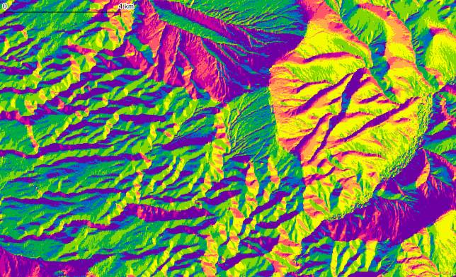
A discrete colour gradient is applied to aspect values (0-359 degrees). The angle ranges and RGB values for the steepest slopes from the Brewer paper were used. Style file available here.

Saturation (Slope)

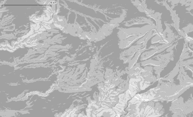
A discrete colour gradient is applied to slope values (0-90 degrees). Flat areas use the same grey value (RGB 161,161,161) as Brewer, with an opacity of 1.0 (255). The opacity of each subsequent step is reduced by 1/3. Style file available here.

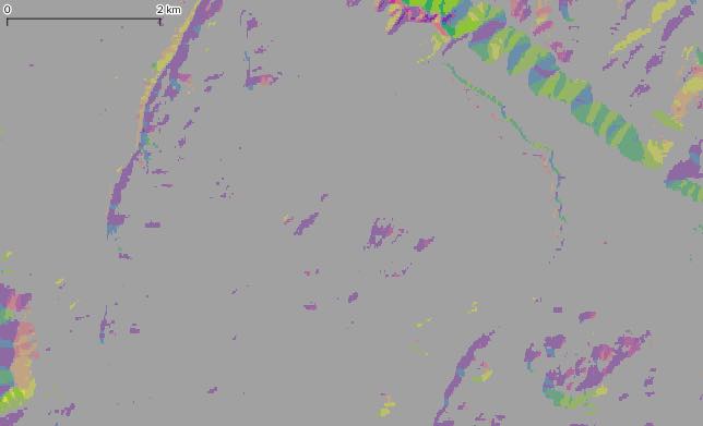
Compositing

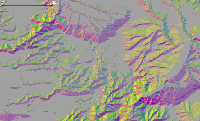
Rendering the slope layer over the aspect layer results in flatter sections being rendered grey, with steep slope sections remaining visible. The results differ slightly from the original implementation as some hand-tweaking of the colour mapping table was performed, and these are not preserved in this method.

Alternative Styles

It’s quite easy with this method to experiment with different rendering techniques.

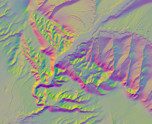
Linear Gradients

The original implementation discretises the aspect/slope gradients. We can also render either/both with linear interpolation between steps. This preserves subtle topographic features at the expense of making specific values harder to determine from the image and increased clutter.

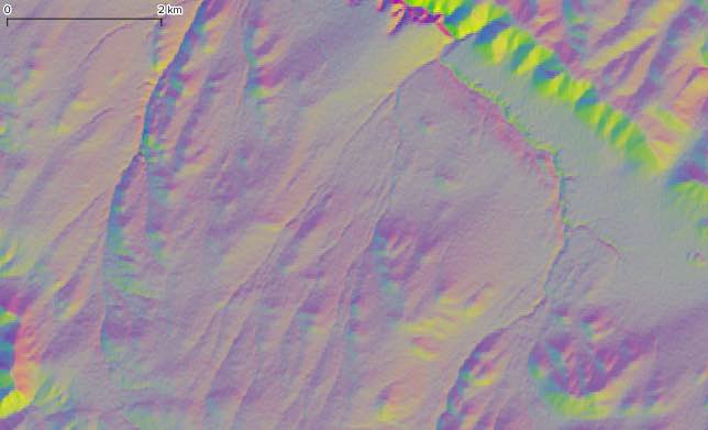
These interpolations are performed in the RGB colour space, and it may be possible to create pleasing results by blending in the HSV or CIE colour spaces.